Tutorial: getting started on simulated data

Mikele Milia, Giacomo Baruzzo and Barbara Di Camillo

This tutorial walks through the complete NEBULA workflow using synthetic data that can be generated entirely within R — no external files or downloads are required. It also documents the exact format that the input files must follow, so that you can apply the same workflow to real datasets.

For installation instructions see the Installation vignette (vignette("installation", package = "nebula")). For running NEBULA inside a container see the Containerized usage vignette (vignette("containers", package = "nebula")).

Overview of the workflow

The standard NEBULA workflow uses three ingredients:

• a genotype dataset in PLINK binary format;
• a collection of SNP-set definitions;
• an analysis directory where null distributions and association results are written.

In practice, the analysis is carried out in three steps:

1. estimate the null hypothesis distribution with compute_null_hypothesis();
2. test SNP-set associations with compute_association();
3. adjust p-values with correct_association().

Required input files

PLINK dataset

The genotype dataset must be provided in PLINK binary format, i.e. as .bed, .bim, and .fam files sharing the same prefix. In NEBULA, root_file_name should be the full path to that prefix, without the file extension.

For example, if the input files are:

/project/data/study.bed
/project/data/study.bim
/project/data/study.fam

then root_file_name should be:

root_file_name <- "/project/data/study"

SNP-set definitions

SNP-sets are groups of SNP identifiers collected according to biological or functional criteria. NEBULA expects:

• a directory containing SNP-set files;
• a tab-delimited list file describing which SNP-sets to analyze.

Each SNP-set file must:

• be named <SNP_SET_NAME>.txt;
• contain 3 tab-delimited columns with no header;
• report SNP, CHR, and BP information for each SNP in the set.

For example, a SNP-set file may look like:

rs123 [TAB] 17 [TAB] 43044295
rs456 [TAB] 17 [TAB] 43047654
rs789 [TAB] 17 [TAB] 43049122

The list file must contain one row per SNP-set in the format:

<SNP_SET_NAME> [TAB] <NUM_SNPS>

For example:

gene_BRCA1 [TAB] 3
gene_TP53 [TAB] 2

An example layout is:

project/
├── data/
│   ├── study.bed
│   ├── study.bim
│   └── study.fam
├── snpsets/
│   ├── gene_BRCA1.txt
│   └── gene_TP53.txt
└── snpset_list.txt

Make sure that the SNP identifiers listed in the SNP-set files match the SNP IDs reported in the PLINK .bim file.

Quick start with synthetic data

If you want to test the full pipeline without downloading external data, NEBULA provides functions to generate a small synthetic dataset and corresponding SNP-sets.

Step 1: simulate genotype data

library(nebula)

root_folder <- "<project-root-folder>"

synthetic_data <- nebula::simulate_synthetic_genotype(
  n_snps = 10,
  n_individuals = 10,
  n_causal_snps = 2
)

head(synthetic_data)

Step 2: save the synthetic dataset in PLINK format

nebula::save_synthetic_genotype(
  synthetic_data,
  file = file.path(root_folder, "synthetic_genotype")
)

This creates PLINK-compatible files with prefix synthetic_genotype.

Step 3: generate synthetic SNP-sets

nebula::generate_synthetic_snpsets(
  input_file = paste0(root_folder, "/synthetic_genotype.bim"),
  snps_per_set = 10,
  num_sets = 10,
  root_dir = root_folder
)

This creates a directory named simulation_10snp and a list file named simulation_10snp_snpsetlist.txt inside root_folder.

After these steps, you can use the synthetic PLINK dataset and generated SNP-set files as input for the full NEBULA workflow.

Run the NEBULA analysis

library(nebula)

root_folder <- "<project-root-folder>"
res_folder <- file.path(root_folder, "results")
dir.create(res_folder, showWarnings = FALSE, recursive = TRUE)

Step 1: estimate the null hypothesis

compute_null_hypothesis() generates the background distribution of entropy scores under the null hypothesis. This step is required before evaluating the observed SNP-set statistics.

nebula::compute_null_hypothesis(
  root_file_name = file.path(root_folder, "synthetic_genotype"),
  pathpathways = file.path(root_folder, "simulation_10snp"),
  pathwaylistfile = file.path(root_folder, "simulation_10snp_snpsetlist.txt"),
  nullhypmsfile = file.path(res_folder, "null_ms.txt"),
  nullhyps2file = file.path(res_folder, "null_s2.txt"),
  seed = 1,
  B = -1,
  alpha = 0.05,
  min_snps = 2,
  max_snps = 999999,
  N_cores = 6,
  n_rows = 10,
  verbosity = 0,
  mode = 0,
  implementation = 0
)

Step 2: test SNP-set association

compute_association() compares the observed SNP-set scores against the null distributions estimated in the previous step.

results <- nebula::compute_association(
  root_file_name = file.path(root_folder, "synthetic_genotype"),
  pathpathways = file.path(root_folder, "simulation_10snp"),
  pathwaylistfile = file.path(root_folder, "simulation_10snp_snpsetlist.txt"),
  nullhypmsfile = file.path(res_folder, "null_ms.txt"),
  nullhyps2file = file.path(res_folder, "null_s2.txt"),
  alpha = 0.05,
  B = -1,
  out_selected = file.path(res_folder, "association_results.txt"),
  min_snps = 2,
  max_snps = 999999,
  N_cores = 6,
  n_rows = 5000,
  verbosity = 0,
  mode = 0,
  association_mode = "MAX"
)

The object returned by compute_association() contains the SNP-set association results and can also be written to disk through out_selected.

Step 3: correct for multiple testing

correct_association() applies multiple-testing correction procedures such as Benjamini-Hochberg and Benjamini-Yekutieli.

corrected_results <- nebula::correct_association(
  results,
  GRCh = "38",
  output_path = res_folder
)

Scalability estimate plot

To help with planning runs on larger datasets, you can build a simple runtime estimate from your input dimensions:

• number of SNPs (n_snps);
• number of individuals (n_individuals);
• number of cores (N_cores);
• chunk size (n_rows, used as the processing chunk parameter).

The model below is intentionally simple and should be treated as an order-of- magnitude estimate, not an exact benchmark. You can calibrate it on your hardware by adjusting calibration_seconds to match one measured run.

In the manuscript (Section 2.6, Eqs. 22 and 30), the dominant time term scales as approximately O(P^2 N / T), where:

• P: number of SNPs;
• N: number of individuals;
• T: number of cores/threads.

Chunk size (C, mapped to n_rows here) mainly affects overhead and memory, rather than the dominant asymptotic term. The estimator below models this via an additional overhead factor proportional to the number of chunks Q = P / C.

estimate_runtime_seconds <- function(
    n_snps,
    n_individuals,
    n_cores,
    n_rows,
    calibration_snps = 10000,
    calibration_individuals = 500,
    calibration_cores = 4,
    calibration_n_rows = 1000,
    calibration_seconds = 120,
    chunk_overhead_weight = 0.2,
    core_efficiency = 0.9
) {
  P <- pmax(n_snps, 1)
  N <- pmax(n_individuals, 1)
  T <- pmax(n_cores, 1)
  C <- pmax(n_rows, 1)

  P0 <- pmax(calibration_snps, 1)
  N0 <- pmax(calibration_individuals, 1)
  T0 <- pmax(calibration_cores, 1)
  C0 <- pmax(calibration_n_rows, 1)

  # Dominant complexity from the manuscript: O(P^2 * N / T)
  dominant_term <- (P^2 * N / T) / (P0^2 * N0 / T0)

  # Real-world correction: less-than-ideal scaling across cores
  core_correction <- (T / (1 + core_efficiency * (T - 1))) /
    (T0 / (1 + core_efficiency * (T0 - 1)))

  # Chunk overhead proxy from Q ~ P/C
  chunk_term <- 1 + chunk_overhead_weight * (P / C)
  chunk_term0 <- 1 + chunk_overhead_weight * (P0 / C0)

  calibration_seconds * dominant_term * (chunk_term / chunk_term0) * core_correction
}

estimate_memory_gb <- function(
    n_snps,
    n_cores,
    n_rows,
    calibration_snps = 10000,
    calibration_cores = 4,
    calibration_n_rows = 1000,
    calibration_memory_gb = 8
) {
  # Memory trend from manuscript (Eq. 31 proxy): O(T * C * P)
  ratio <- (pmax(n_cores, 1) * pmax(n_rows, 1) * pmax(n_snps, 1)) /
    (pmax(calibration_cores, 1) * pmax(calibration_n_rows, 1) * pmax(calibration_snps, 1))

  calibration_memory_gb * ratio
}

format_plain <- function(x, digits = 2) {
  format(round(x, digits), big.mark = ",", scientific = FALSE, trim = TRUE)
}

label_snps <- function(x) {
  x_chr <- format(x, scientific = FALSE, trim = TRUE)
  dplyr::case_when(
    x_chr == "10000" ~ "10K",
    x_chr == "50000" ~ "50K",
    x_chr == "100000" ~ "100K",
    x_chr == "200000" ~ "200K",
    TRUE ~ x_chr
  )
}

scenario_grid <- expand.grid(
  n_snps = c(10000, 50000, 100000, 200000),
  n_individuals = c(500, 1000, 2000, 5000),
  n_cores = c(1, 2, 4, 8, 16, 32),
  n_rows = c(250, 500, 1000, 2000),
  KEEP.OUT.ATTRS = FALSE,
  stringsAsFactors = FALSE
)

scenario_grid$runtime_minutes <- estimate_runtime_seconds(
  n_snps = scenario_grid$n_snps,
  n_individuals = scenario_grid$n_individuals,
  n_cores = scenario_grid$n_cores,
  n_rows = scenario_grid$n_rows
) / 60

scenario_grid$memory_gb <- estimate_memory_gb(
  n_snps = scenario_grid$n_snps,
  n_cores = scenario_grid$n_cores,
  n_rows = scenario_grid$n_rows
)

scenario_grid$n_snps_label <- factor(
  label_snps(scenario_grid$n_snps),
  levels = c("10K", "50K", "100K", "200K")
)

scenario_grid$n_individuals_label <- factor(
  scenario_grid$n_individuals,
  levels = c(500, 1000, 2000, 5000)
)

scenario_grid$chunk_label <- factor(
  paste0("Chunk = ", format_plain(scenario_grid$n_rows, digits = 0)),
  levels = paste0("Chunk = ", c("250", "500", "1,000", "2,000"))
)

if (requireNamespace("ggplot2", quietly = TRUE)) {
  ggplot2::ggplot(
    scenario_grid,
    ggplot2::aes(
      x = runtime_minutes,
      y = memory_gb,
      color = n_snps_label,
      shape = n_individuals_label,
      size = n_cores
    )
  ) +
    ggplot2::geom_point(alpha = 0.8, stroke = 0.25) +
    ggplot2::facet_wrap(~chunk_label, ncol = 2) +
    ggplot2::scale_x_log10(labels = function(x) format_plain(x, digits = 1)) +
    ggplot2::scale_y_log10(labels = function(y) format_plain(y, digits = 1)) +
    ggplot2::scale_color_manual(values = c("10K" = "#1b9e77", "50K" = "#d95f02", "100K" = "#7570b3", "200K" = "#e7298a"), drop = FALSE) +
    ggplot2::scale_shape_manual(values = c("500" = 16, "1000" = 17, "2000" = 15, "5000" = 3), drop = FALSE) +
    ggplot2::scale_size_continuous(range = c(2.2, 6.5), breaks = c(1, 2, 4, 8, 16, 32)) +
    ggplot2::labs(
      title = "Estimated NEBULA scalability",
      subtitle = "Time and memory estimates derived from the complexity model in the manuscript",
      x = "Estimated runtime (minutes)",
      y = "Estimated memory (GB)",
      color = "SNPs (P)",
      shape = "Individuals (N)",
      size = "Cores (T)"
    ) +
    ggplot2::theme_minimal(base_size = 11) +
    ggplot2::theme(
      legend.position = "right",
      panel.grid.minor = ggplot2::element_blank(),
      strip.text = ggplot2::element_text(face = "bold")
    )
} else {
  message("Package 'ggplot2' not installed: install it to render the faceted scatter plot.")
}

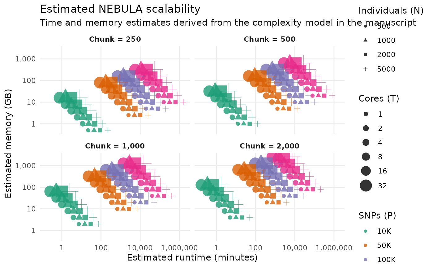
For your project, update input with your expected run configuration. If you benchmark one real run, set calibration_seconds to that runtime to make the estimates more realistic for your machine.

Recommended project structure

For reproducible analyses, it is useful to keep inputs and outputs organized in a simple folder layout such as:

project/
├── data/
│   ├── synthetic_genotype.bed
│   ├── synthetic_genotype.bim
│   └── synthetic_genotype.fam
├── snpsets/
├── results/
└── snpset_list.txt

Summary

NEBULA analyses can be organized around a straightforward sequence:

1. prepare a PLINK dataset and a set of SNP-set definitions;
2. generate null distributions with compute_null_hypothesis();
3. run the association analysis with compute_association();
4. adjust p-values with correct_association().

When external data are not available, the synthetic data utilities provide a convenient way to test the entire workflow end-to-end.